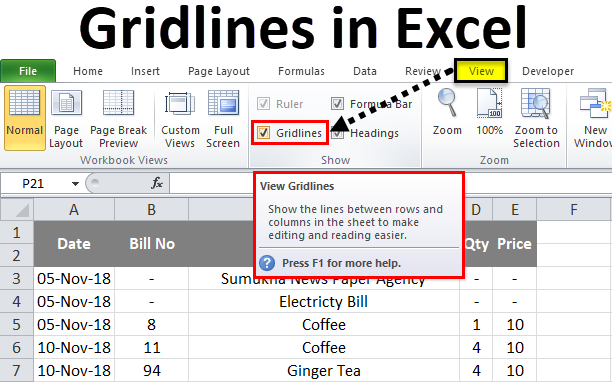
How to Hide Gridlines in Microsoft Excel

Microsoft Excel is a great tool for managing data, making calculations, and creating charts and graphs. However, when working with large amounts of data, it can be confusing and distracting to see the gridlines on your worksheet. Fortunately, it is easy to hide gridlines in Excel. Read on to learn how to do it.
Method 1: Using the Ribbon
Step 1: Open your Excel worksheet.
Step 2: Click on the “View” tab on the ribbon.
Step 3: In the “Show” group, uncheck the “Gridlines” option.
Method 2: Using the Cell Format
Step 1: Open your Excel worksheet.
Step 2: Select the cells in which you want to hide the gridlines.
Step 3: Right-click on the selection and choose “Format Cells.”
Step 4: In the “Format Cells” dialog box, click on the “Border” tab.
Step 5: Under “Presets”, choose “No border.”
Step 6: Click “OK” to close the dialog box.
The gridlines will now be hidden in the selected cells.
Method 3: Using the Excel Options
Step 1: Open your Excel worksheet.
Step 2: Click on the “File” tab on the ribbon.
Step 3: Click on “Options.”
Step 4: In the “Excel Options” dialog box, click on “Advanced.”
Step 5: Scroll down to the “Display options for this worksheet” section.
Step 6: Uncheck the “Show gridlines” option.
Step 7: Click “OK” to apply the changes.


