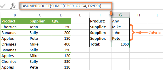
Excel SUMIFS: How to Sum Only Values Meeting Multiple Criteria

Excel is a powerful tool that helps people perform various calculations and data analysis operations. One of the most useful functions in Excel is SUMIFS. This function allows users to sum values based on multiple criteria, making it easy to filter and analyze data efficiently. In this article, we’ll explore the basics of SUMIFS and show you how to use it to sum only values that meet multiple criteria.
What is SUMIFS in Excel?
SUMIFS is a function in Excel that allows users to add values together based on multiple criteria. By using the SUMIFS function, users can create complex calculations that filter data based on various conditions. This function is especially helpful when dealing with large datasets, where it can be challenging to sift through the data manually.
To use the SUMIFS function, users must specify the range of cells to sum, followed by the criteria they want to use to filter the data. The function requires at least one range and one criteria, but users can add additional ranges and criteria based on their needs.
How to use SUMIFS to Sum Only Values Meeting Multiple Criteria
The SUMIFS function is incredibly versatile and can be used in many different ways. One common way people use this function is to add values together based on multiple criteria. Here are the steps to follow to use SUMIFS to sum only values meeting multiple criteria:
1. Define the ranges
The first thing you need to do is to define the ranges you want to use in the function. For example, if you have a dataset with columns A, B, and C, you may want to sum the values in column C, based on criteria in columns A and B. In this case, you would define the ranges as follows:
=SUMIFS(C:C, A:A, criteria1, B:B, criteria2)
2. Set the criteria
Next, you need to set the criteria for each range. Criteria are the conditions you want to use to filter the data. For example, you might want to sum only the values in column C where the values in column A are equal to “Apples,” and the values in column B are equal to “Red.”
In this case, you would set the criteria as follows:
=SUMIFS(C:C, A:A,”Apples”, B:B,”Red”)
This would tell Excel to sum only the values in column C where the values in column A are “Apples,” and the values in column B are “Red.”
3. Add additional criteria (optional)
You can add additional criteria as needed to further filter the data. For example, if you wanted to add a third criterion, such as a date range, you would add an additional range and criteria to the function:
=SUMIFS(C:C, A:A,”Apples”, B:B,”Red”, D:D,”>=1/1/2022″, D:D,”<=6/30/2022″)
This would tell Excel to sum only the values in column C where the values in column A are “Apples,” the values in column B are “Red,” and the values in column D fall between 1/1/2022 and 6/30/2022.
Conclusion
The SUMIFS function is an incredibly powerful tool that can save users time and effort when working with large datasets. By using the function to filter data based on multiple criteria, users can quickly perform complex calculations and analysis. With the steps outlined in this article, you can use the SUMIFS function to sum only values meeting multiple criteria, making it easier to analyze your data and draw meaningful insights.


